
Binomial Tree
Introduction
The Financial Risk Manager (FRM®) introduces binomial trees by applying them to value derivatives for two asset classes, equities and bonds. For stock options, the text is John Hull’s Options, Futures and Derivatives; for bonds, the text is Bruce Tuckman’s Fixed Income Securities. Both are excellent and have been assigned in the syllabus for years.
What are the virtues of a binomial tree? I think the first advantage is simply that a binomial tree is highly intuitive. It is a map of future possible outcomes: rather than project a single future, many possible paths can be articulated. The second advantage is their flexibility. Unlike the Black-Scholes-Merton which is analytically elegant but requires us to submit to a set of assumptions, the binomial tree can be constructed according to all sorts of assumptions (including it can be “extended” to a trinomial tree).
To utilize a binomial tree, there are three essential steps:
- Specify the assumptions.
- Build the tree forward by valuing the future nodes.
- And, finally, works backwards to the present to value the derivative.
First Step: Specify Assumptions
In order to build the binomial tree forward, we need to first specify the dynamic of the underlying risk factor. In the FRM, the risk factor tends to be an asset price (e.g., stock price) or an interest rate. I use the term “risk factor” to remind us that, while we are conducing a valuation of a derivative, in risk we tend to view prices or rates as risk factors, also. In this post, I won’t be covering the deep topic of interest rate dynamics. Instead, I will just look at an equity call option.
The key to our assumptions are the magnitude of the up (u) and down (d) jumps and the probability of an up jump (p). Hull first introduces a simple assumption of +/- 10%; that is, u = 1.10 and d = 0.90. Similarly +/- 20% implies u = 1.20 and d = 0.80. We might think of this (very loosely) as approximating prices with a normal distribution. If a $10.00 stock moves up in two consecutive steps, then the final price is $10.00 * 1.2 * 1.2 = $14.40. But notice an interesting outcome. If the stock moves up then down (or down then up) we don’t finish back where we started, we finish slightly lower: $10.00 * 1.20 * 0.80 = $9.60.
A more sophisticated assumption is to “match volatility with u and d,” as Hull puts it. This means that a volatility assumption informs the (u) and (d). This has theoretical benefits including it implicitly matches the Black-Scholes assumption that prices are lognormal; this is the assumption that–as we increase the model’s step–will converge on the Black-Scholes value.
Below are assumptions and a simple four-step binomial tree for a European call option with a maturity of one year:
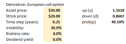
My assumptions are in yellow. Let me clarify a few items:
- Our time step is 0.25 years because we have four steps over one year; I.e., one year divided by four steps equals 0.25 years per step.
- Up(u)= exp[σ*sqrt(Δt)] = exp[volatility*sqrt(time step)] = 1.1618exp(30%*sqrt[0.25]) = 1.1618
- Down(d) = exp[-σ*sqrt(Δt)] = exp[-volatility*sqrt(time step)] = 1/u = 0.8607
- Probability(p) = (exp[(r-q)*Δt]-d)/(u-d) = 0.495945; therefore, the probability of a down move = 1 – p = 0.504055
Second Step: Build the Tree Forward
Given those assumptions, here is the implied binomial tree:

Notice this binomial tree is a recombining tree. That means that the exact sequence of ups and downs does not matter. The stock can jump up to 34.86 then down to 30.00, which is the same value as jumping down to 25.82 then up to 30.00; i.e, ud = du. The initial price of $30.00 is located at node[0,0]. A jump up to node[1,1] returns a value of $34.86 = $30.00*u. A jump down to node[1,0] returns a value of $25.82 = $30.00*d. Consider the $40.50 at node[4,4]. It can be reached via four paths: uuud, uudu, uduu, and duuu. That’s a binomial coefficient. In Excel, COMBIN(number = 4, number_chosen = 3) = 4, because there are four ways to select three up jumps from four jumps. I added the final blue column because that’s the binomial distribution which characterized the final distribution of price outcomes; e.g., there is 24.6% probability that the final price will reach $40.50. We can get this probability by multiplying four (4) by p^3*(1-p)^1; I.e., BINOM.DIST(number_s = 3, trials = 4, p = 0.4959, cumulative = false = 0.246
Third Step: Backward Induction
Now we work backwards, starting from the nodes at maturity. But please note we are switching from stock prices (above) to option prices (below):

At node[4,4] the terminal option value is the option’s intrinsic value at maturity: $54.66 stock price minus $20.00 stock price. The value of the final five nodes is MAX(0,S-K).
How do we calculate node[3,3] = $27.25? It is not the option’s intrinsic value at this time because this is a European option; it cannot be exercised in nine months! Rather, this is the discounted expected value, such that $27.25 = [(p*34.66)*(1-p)*20.50]*exp(-0.04*0.25). The other nodes are similarly induced backwardly, until we get the present option value of $11.00 = [(p*15.45)*(1-p)*6.85]*exp(-0.04*0.25). Notice that’s appropriately greater than the option’s current intrinsic value of $10.00; this option has about $1.00 of time value.
American Style Options
I mentioned a key advantage of the binomial is its flexibility. This includes its ability to naturally model American-style options which can be exercised prior to maturity. The solution is simply to modify each node to return MAX(discounted expected value, intrinsic value). In other words, if the node’s intrinsic value exceeds its discounted expected value, the binomial “assumes” the holder will exercise.
To illustrate, let’s assume an American-style put option and its implied stock price tree:

Below compare the option values at each node, discounted expected value (below left) and intrinsic value (below right):

If this were a European put option, the option’s price would be $1.89; i.e., the discounted expected value. But, if the option is American-style, then each node—except for the final nodes which all must be intrinsic value at maturity—is given by the MAX(discounted expected value, intrinsic value). Notice node[3,0]. It’s intrinsic value of $7.99 exceeds its discounted expected value of $7.73.
Therefore it is assumed for the node’s value and the American-style tree looks like this:
")
The “revised” option price is $1.93 which is higher than $1.89. Indeed, an American style must be worth more than the corresponding European put.
Summary
If you would like to explore these trees further, here is my spreadsheet .
We’ve just scratched the surface but this introduces the fundamentals. The assigned text (John Hull’s Options Futures and other Derivatives gives a much more detailed introduction.
I am also fond of Kolb’s Competing Text Futures, Options and Swaps , which in my opinion is a slightly deeper introduction in some respects. Please feel free to engage me with questions or join the forum conversation if you want to talk about the binomial further!